LaTeX

From Python Code to Mathematical Notation: A Practical Guide to Understanding and Writing LaTeX Formulas

Rajiv KumarSeptember 16, 20266 min read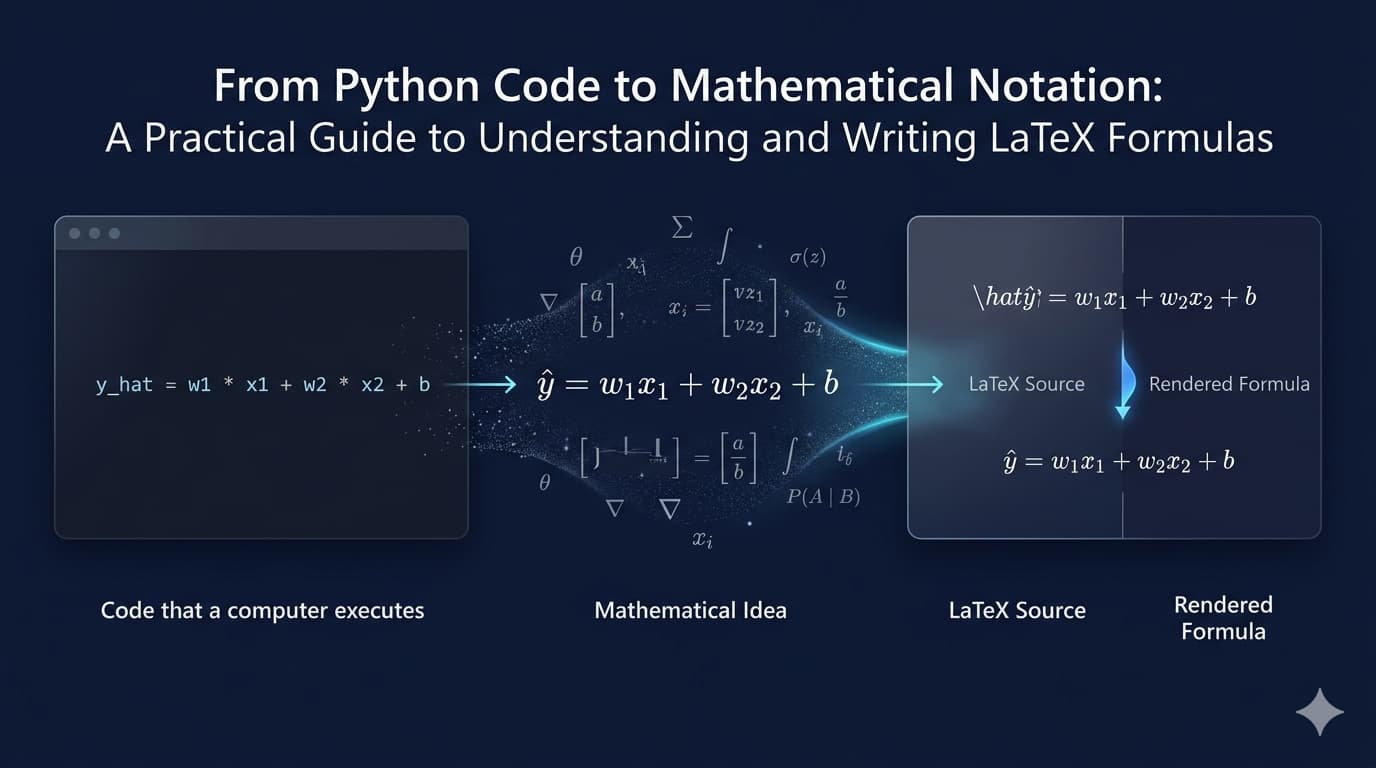

From Python Code to Mathematical Notation: A Practical Guide to Understanding and Writing LaTeX Formulas

Mathematics and programming often describe the same idea in two different languages.A mathematics textbook may write: A Python developer may write:y_hat = w1 * x1 + w2 * x2 + bBoth expressions…

Mathematics and programming often describe the same idea in two different languages.

A mathematics textbook may write:

y\hat{} ​=h_θ​(x)=w_1​x_1​+w_2​x_2​+⋯+w_n​x_n​+b

A Python developer may write:

y_hat = w1 * x1 + w2 * x2 + b

Both expressions represent the same basic calculation. The difference is that the mathematical version is designed for human reading, while the Python version is designed for execution by a computer.

Understanding this difference is important for anyone learning:

Python
Machine Learning
Artificial Intelligence
Statistics
Data Science
Deep Learning
Mathematics for Computer Science
Technical documentation
Research papers
Jupyter Notebooks
AI and software engineering

LaTeX provides a bridge between these two worlds. It allows us to write mathematical notation in plain text and convert it into the professionally typeset formulas commonly seen in mathematics books, research papers, technical documentation, and educational content.

This article explains how to read mathematical LaTeX, how the same formula is written in Python, what output Python produces, and how the LaTeX source becomes a rendered mathematical expression.

1. Mathematics, Python, and LaTeX Describe the Same Idea Differently

Consider this mathematical expression:

y = 2x + 3

It means:

Multiply $x$ by $2$ .
Add 3.
Store the result in $y$ .

The same calculation in Python is:

x = 5
y = 2 * x + 3

print(y)

Python Output:

The Python interpreter executes the instructions and calculates the result.

However, if we want to explain the formula in a technical article, a mathematical textbook, or a research paper, we may prefer the following LaTeX source:

Latex

y = 2x + 3

Rendered LaTeX result

y = 2x + 3

The three versions have different purposes:

Format	Purpose
Python code	Executes the calculation
Python output	Shows the calculated result
LaTeX source	Describes how the mathematical expression should be typeset
Rendered formula	Displays the mathematical expression visually

2. Why Should a Python Developer Learn Mathematical LaTeX?

Learning LaTeX is not mandatory for writing Python programs. You can become a Python developer without knowing LaTeX.

However, LaTeX becomes very useful when you work with mathematical or technical content.

1.1 Machine Learning formulas are usually written in mathematical notation

Machine Learning contains many formulas involving:

Greek letters
Subscripts
Superscripts
Fractions
Summations
Integrals
Matrices
Probability notation
Derivatives
Vectors
Optimization functions

For example, a linear regression model may be written as:

y\hat{} ​=h_θ​(x)=w_1​x_1​+w_2​x_2​+⋯+w_n​x_n​+b

Writing the same expression in Python may look like this:

y_hat = w1 * x1 + w2 * x2 + ... + wn * xn + b

n real Python code, the ellipsis is normally not used for an actual calculation. We would usually use a loop, a list, or a numerical library:

y_hat = sum(w * x for w, x in zip(weights, features)) + b

1.2 LaTeX helps you understand formulas instead of memorizing symbols

When you see:

\hat{y} = h_{\theta}(x)

you can understand the structure:

\hat{y} creates a hat over y
h_{\theta} creates a subscript containing the Greek letter theta
(x) indicates that the function receives x

The rendered result is:

\hat{y}=h_{\theta}(x)

\hat{y} → $\hat{y}$

\theta → $\theta$

\mid → $\mid$

\text{Spam} → $\text{Spam}$

\cdot → $\cdot$

\frac{a}{b} → $\frac{a}{b}$

2. Superscript aur Subscript

LaTeX	Result	Meaning
x^2	$x^2$	Power
x^n	$x^n$	Power
x_i	$x_i$	Subscript
x_{ij}	$x_{ij}$	Multiple-character subscript
x^{2n}	$x^{2n}$	Multiple-character superscript
x_i^2	$x_i^2$	Both
x_{i,j}	$x_{i,j}$	Complex subscript

3. Accent aur Special Marks

LaTeX	Result	Use
\hat{y}	$\hat{y}$	Estimated value
\bar{x}	$\bar{x}$	Mean/average
\vec{v}	$\vec{v}$	Vector
\dot{x}	$\dot{x}$	First derivative
\ddot{x}	$\ddot{x}$	Second derivative
\tilde{x}	$\tilde{x}$	Approximation
\overline{AB}	$\overline{AB}$	Line/average
\underline{x}	$\underline{x}$	Underline
\widehat{ABC}	$\widehat{ABC}$	Wide hat
\widetilde{ABC}	$\widetilde{ABC}$	Wide tilde

4. Greek Letters

LaTeX	Result	LaTeX	Result
\alpha	$\alpha$	\beta	$\beta$
\gamma	$\gamma$	\delta	$\delta$
\epsilon	$\epsilon$	\varepsilon	$\varepsilon$
\zeta	$\zeta$	\eta	$\eta$
\theta	$\theta$	\vartheta	$\vartheta$
\iota	$\iota$	\kappa	$\kappa$
\lambda	$\lambda$	\mu	$\mu$
\nu	$\nu$	\xi	$\xi$
\pi	$\pi$	\varpi	$\varpi$
\rho	$\rho$	\varrho	$\varrho$
\sigma	$\sigma$	\varsigma	$\varsigma$
\tau	$\tau$	\upsilon	$\upsilon$
\phi	$\phi$	\varphi	$\varphi$
\chi	$\chi$	\psi	$\psi$
\omega	$\omega$	\Gamma	$\Gamma$

4.1 Uppercase Greek letters

LaTeX	Result	LaTeX	Result
\Gamma	$\Gamma$	\Delta	$\Delta$
\Theta	$\Theta$	\Lambda	$\Lambda$
\Xi	$\Xi$	\Pi	$\Pi$
\Sigma	$\Sigma$	\Upsilon	$\Upsilon$
\Phi	$\Phi$	\Psi	$\Psi$
\Omega	$\Omega$

5. Fractions

In the fraction uses numerator and denominator "\frac{numerator}{denominator}" → $\frac{numerator}{denominator}$

\frac{a}{b} → $\frac{a}{b}$

\frac{x+1}{x-1} → $\frac{x+1}{x-1}$

\frac{P(W \mid \text{Spam}) \cdot P(\text{Spam})}{P(W)} → $\frac{P(W \mid \text{Spam}) \cdot P(\text{Spam})}{P(W)}$

5.1 Nested Fraction

\frac{1}{1+\frac{a}{b}} → $\frac{1}{1+\frac{a}{b}}$

6. Multiplication

LaTeX	Result	Meaning
ab	$ab$	Normal multiplication
a b	$ab$	Spacing ignored
a \cdot b	$a \cdot b$	Center dot
a \times b	$a \times b$	Cross multiplication
a \ast b	$a \ast b$	Asterisk
a \star b	$a \star b$	Star operator

7. Relations aur Comparison Symbols

LaTeX	Result
=	$=$
\neq	$\neq$
\ne	$\ne$
<	$<$
>	$>$
\leq	$\leq$
\geq	$\geq$
\approx	$\approx$
\sim	$\sim$
\simeq	$\simeq$
\equiv	$\equiv$
\propto	$\propto$
\ll	$\ll$
\gg	$\gg$

Examples:

x \geq 0 → $x \geq 0$

P(A) \approx P(B) → $P(A) \approx P(B)$

y \propto x → $y \propto x$

8. Probability Symbols

LaTeX	Result	Meaning
P(A)	$P(A)$	Probability
P(A \mid B)	$P(A \mid B)$	Conditional probability
P(A \cap B)	$P(A \cap B)$	Intersection
P(A \cup B)	$P(A \cup B)$	Union
P(A^c)	$P(A^c)$	Complement
P(\neg A)	$P(\neg A)$	Not A
\mid	$\mid$	Given/conditional
\Pr(A)	$\Pr(A)$	Probability notation

Dynamic-size brackets

\left(\frac{a}{b}\right) → $\left(\frac{a}{b}\right)$

9. Set Theory Symbols

LaTeX	Result	Meaning
\in	$\in$	Belongs to
\notin	$\notin$	Does not belong
\subset	$\subset$	Subset
\subseteq	$\subseteq$	Subset or equal
\supset	$\supset$	Superset
\emptyset	$\emptyset$	Empty set
\varnothing	$\varnothing$	Empty set
\mathbb{R}	$\mathbb{R}$	Real numbers
\mathbb{N}	$\mathbb{N}$	Natural numbers
\mathbb{Z}	$\mathbb{Z}$	Integers
\mathbb{Q}	$\mathbb{Q}$	Rational numbers
\mathbb{C}	$\mathbb{C}$	Complex numbers
\cup	$\cup$	Union
\cap	$\cap$	Intersection

Example

x \in \mathbb{R} → $x \in \mathbb{R}$

A \subseteq B → $A \subseteq B$

11. Summation, Product and Calculus

Summation	\sum_{i=1}^{n} x_i	$\sum_{i=1}^{n} x_i$
Product	\prod_{i=1}^{n} x_i	$\prod_{i=1}^{n} x_i$
Definite integral	\int x^2 \, dx	$\int x^2 \, dx$
Partial derivative	\frac{\partial f}{\partial x}	$\frac{\partial f}{\partial x}$
Normal derivative	\frac{dy}{dx}	$\frac{dy}{dx}$
Gradient	\nabla f	$\nabla f$
Limit	\lim_{x \to 0} f(x)	$\lim_{x \to 0} f(x)$
Infinity	\infty	$\infty$

12. Logic Symbols

LaTeX	Result	Meaning
\land	$\land$	AND
\lor	$\lor$	OR
\neg	$\neg$	NOT
\Rightarrow	$\Rightarrow$	Implies
\Leftarrow	$\Leftarrow$	Implied by
\Leftrightarrow	$\Leftrightarrow$	If and only if
\forall	$\forall$	For all
\exists	$\exists$	Exists
\nexists	$\nexists$	Does not exist

Example

A \Rightarrow B	$A \Rightarrow B$
\forall x \in \mathbb{R}.	$\forall x \in \mathbb{R}.$

13. Arrows

Tip

x \to \infty

$x \to \infty$

LaTeX	Result
\to	$\to$
\rightarrow	$\rightarrow$
\leftarrow	$\leftarrow$
\Rightarrow	$\Rightarrow$
\Leftarrow	$\Leftarrow$
\leftrightarrow	$\leftrightarrow$
\Leftrightarrow	$\Leftrightarrow$
\uparrow	$\uparrow$
\downarrow	$\downarrow$
\mapsto	$\mapsto$

14. Vectors, Matrices aur Linear Algebra

Vector

\mathbf{x}	$\mathbf{x}$
\vec{x}	$\vec{x}$

Matrix

\begin{bmatrix} a & b \\ c & d \end{bmatrix}	$\begin{bmatrix} a & b \\ c & d \end{bmatrix}$
\begin{matrix} a & b \\ c & d \end{matrix}	$\begin{matrix} a & b \\ c & d \end{matrix}$
\begin{pmatrix} a & b \\ c & d \end{pmatrix}	$\begin{pmatrix} a & b \\ c & d \end{pmatrix}$
\begin{vmatrix} a & b \\ c & d \end{vmatrix}	$\begin{vmatrix} a & b \\ c & d \end{vmatrix}$
A = [a_{ij}]_{m \times n}	$A = [a_{ij}]_{m \times n}$

15. Common ML Formula Patterns

Linear regression	\hat{y} = w_1x_1 + w_2x_2 + \cdots + w_nx_n + b	$\hat{y} = w_1x_1 + w_2x_2 + \cdots + w_nx_n + b$
Vector form	\hat{y} = \mathbf{w}^{T}\mathbf{x} + b	$\hat{y} = \mathbf{w}^{T}\mathbf{x} + b$
Sigmoid function	\sigma(z) = \frac{1}{1 + e^{-z}}	$\sigma(z) = \frac{1}{1 + e^{-z}}$
Mean squared error	\mathrm{MSE} = \frac{1}{n}\sum_{i=1}^{n}(y_i-\hat{y}_i)^2	$\mathrm{MSE} = \frac{1}{n}\sum_{i=1}^{n}(y_i-\hat{y}_i)^2$
Gradient descent	\theta := \theta - \alpha \nabla_{\theta} J(\theta)	$\theta := \theta - \alpha \nabla_{\theta} J(\theta)$
Bayes theorem	P(A \mid B) = \frac{P(B \mid A)P(A)}{P(B)}	$P(A \mid B) = \frac{P(B \mid A)P(A)}{P(B)}$
Expected value	\mathbb{E}[X]	$\mathbb{E}[X]$
Variance	\operatorname{Var}(X)	$\operatorname{Var}(X)$
Norm	\\|\mathbf{x}\\|_2	$\\|\mathbf{x}\\|_2$
Dot product	\mathbf{x} \cdot \mathbf{y}	$\mathbf{x} \cdot \mathbf{y}$

16. Spacing Commands

LaTeX	Use
\,	Small space
\:	Medium space
\;	Large space
\quad	Large horizontal space
\qquad	Extra-large space
\!	Negative space

Example

\int x^2 \, dx → $\int x^2 \, dx$

17. Special Characters

LaTeX	Result
\%	$\%$
\$	$\$$
\&	$\&$
\#	$\#$
\_	$\_$
\{	$\{$
\}	$\}$
\textbackslash	Backslash

Example

\text{Accuracy} = 95\% $\text{Accuracy} = 95\%$

18. Cases / Piecewise Function and Aligned Equations

Example

Piecewise Function	f(x) = \begin{cases} x^2, & x \geq 0 \\ -x, & x < 0 \end{cases}	$f(x) = \begin{cases} x^2, & x \geq 0 \\ -x, & x < 0 \end{cases}$
Aligned Equations	\begin{aligned} y &= mx + b \\ &= 2x + 3 \end{aligned}	$\begin{aligned} y &= mx + b \\ &= 2x + 3 \end{aligned}$

Piecewise Function

f(x) =

\begin{cases}

x^2, & x \geq 0 \\

-x, & x < 0

\end{cases}

$f(x) = \begin{cases} x^2, & x \geq 0 \\ -x, & x < 0 \end{cases}$

Aligned Equations

\begin{aligned}

y &= mx + b \\

&= 2x + 3

\end{aligned}

$\begin{aligned} y &= mx + b \\ &= 2x + 3 \end{aligned}$

19. important 25 commands for ML

1. ^

2. _

3. \hat{}

4. \bar{}

5. \mathbf{}

6. \theta

7. \sigma

8. \mu

9. \sum

10. \prod

11. \int

12. \frac{}{}

13. \cdot

14. \times

15. \mid

16. \text{}

17. \left

18. \right

19. \in

20. \mathbb{}

21. \nabla

22. \partial

23. \approx

24. \leq

25. \geq

Prompt Engineering

Write the Handoff Before You Close the AI Session

Aug 11, 2026·11 min read

Prompt Engineering

The Project Brief Every AI Coding Session Should Read First

Aug 11, 2026·10 min read

Prompt Engineering

Giving an AI Assistant Project Memory That Survives the Session

Aug 11, 2026·12 min read

1. Mathematics, Python, and LaTeX Describe the Same Idea Differently

1.1 Machine Learning formulas are usually written in mathematical notation

1.2 LaTeX helps you understand formulas instead of memorizing symbols

2. Superscript aur Subscript

3. Accent aur Special Marks

4. Greek Letters

4.1 Uppercase Greek letters

5. Fractions

5.1 Nested Fraction

6. Multiplication

7. Relations aur Comparison Symbols

Examples:

8. Probability Symbols

9. Set Theory Symbols

11. Summation, Product and Calculus

12. Logic Symbols

13. Arrows

14. Vectors, Matrices aur Linear Algebra

15. Common ML Formula Patterns

16. Spacing Commands

17. Special Characters

18. Cases / Piecewise Function and Aligned Equations

19. important 25 commands for ML

Related articles

Write the Handoff Before You Close the AI Session

The Project Brief Every AI Coding Session Should Read First

Giving an AI Assistant Project Memory That Survives the Session